Introduction
-
Two indices are used to evaluate the accuracy of a test that predicts dichotomous outcomes (
e.g.
logistic regression) - sensitivity and specificity. They describe how well a test discriminates between cases with and without a certain condition.
Sensitivity - the proportion of true positives or the proportion of cases correctly identified by the test as meeting a certain condition (e.g. in mammography testing, the proportion of patients with cancer who test positive).Choosing a Cut-off
Specificity - the proportion of true negatives or the proportion of cases correctly identified by the test as not meeting a certain condition (e.g. in mammography testing, the proportion of patients without cancer who test negative).
The position of the cut-off determines the number of true positives, true negatives, false positives, and false negatives. As you increase your sensitivity (true positives) and can identify more cases with a certain condition, you also sacrifice accuracy on identifying those without the condition (specificity).
For a clinical example and graphical description see the University of Nebraska Medical Center Web Site: Introduction to ROC Curves: http://gim.unmc.edu/dxtests/ROC1.htm
Receiver Operating Characteristic (ROC) Curve
-
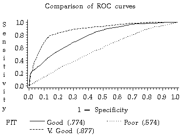
A Receiver Operating Characteristic (ROC) curve is a graphical representation of the trade off between the false negative and false positive rates for every possible cut off. By tradition, the plot shows the false positive rate (1-specificity) on the X axis and the true positive rate (sensitivity or 1 - the false negative rate) on the Y axis. See
"Professor Mean's explanation of the ROC Curve"
below.
The accuracy of a test (i.e. the ability of the test to correctly classify cases with a certain condition and cases without the condition) is measured by the area under the ROC curve. An area of 1 represents a perfect test, while an area of .5 represents a worthless test. The closer the curve follows the left-hand border and then the top border of the ROC space, the more accurate the test; the true positive rate is high and the false positive rate is low. Statistically, more area under the curve means that it is identifying more true positives while minimizing the number/percent of false positives.

Sample SAS Code for Graphing an ROC Curve
-
The LOGISTIC procedure in SAS includes an option to output the sensitivity and specificity of any given model at different cutoff values. From this dataset an ROC curve can be graphed.
The SAS code below estimates a logistic model predicting 30-day mortality following AMI in Manitoba over 3 years.
proc logistic data=ami descending;
model dth30 = age5064 age6574 age75p nsex shock diabcomp chf malig cvd pulmoned renal1 renal2 carddys / outroc=rocdata;
title1 'Predicting 30-day mortality, MB AMI, F94-96';
run;
The option OUTROC= (line 4) specifies the name of the dataset containing the ROC curve data.
This can then be plotted using PROC GPLOT:
proc gplot data=rocdata;The variables _SENSIT_ and _1MSPEC_ are the sensitivity and 1-specificity values which, when plotted against each other, produce the ROC curve.
plot _sensit_*_1mspec_;
title1 h=1.5 'ROC curve: AMI data';
run;
quit;