1996 Census Enumeration Area Level Average Household Income

The 1996 census was released by the Data Liberation Initiative in stages starting in October 1997 and completing in July 1998. The component reporting sources of income, family and household income at the enumeration area level was released on June 12, 1998. This file, entitled 'Beyond 2020', was supplied by Statistics Canada. The file contained the following variables:


1. Level of geography (province/federal electoral district/enumeration area)
   
2. Population 15 years and older
   
3. Population 15 years and older without income
   
4. Population 15 years and older with income
   
5. Average 1995 income in dollars
   
6. Standard error of average income in dollars
   
7. Number of private households
   
8. Average household income of all private households in dollars
   
9. Standard error of average household income in dollars

This file contains 1,764 records, 1 record at the province level, 14 records at the federal electoral district level and 1,749 records at the enumeration area level. In addition to the enumeration area level average household income file, I also created a census subdivision area level text file of average household income and an enumeration area level text file of population.

Suppression of Average Household Income

To protect the confidentiality of individual responses Statistics Canada has adopted a technique known as area suppression. Area suppression is the deletion of all characteristic data for geographic areas with populations below a specified size. The extent to which data are suppressed depends upon the following factors:


• If the data are tabulated from the 100% database, the data are suppressed if the total population in the area is less than 40.
  
  
• If the data are tabulated from the 20% sample database, the data are suppressed if the total non-institutional population in the area from either the 100% or 20% databases is less than 40.

Exceptions to these rules:


• Income distributions and related statistics are suppressed if the total non-institutional population in the area from either the 100% or 20% databases is less than 250.
  
  
• If the data are tabulated from the 100% database and refer to six-character postal codes, the data are suppressed if the total population in the area is less than 100.
  
  
• If the data are tabulated from the 20% sample database and refer to six-character postal codes, the data are suppressed if the total non- institutional population in the area from either the 100% or 20% databases is less than 100.

The enumeration area level and the census subdivision level average household income files are both subject to the minimum 250 non-institutional population suppression rule. The following table describes the degree to which suppression has taken place on the enumeration area level file:

Table 1: Degree of Suppression



CSD	Number of EAs	Population Aged 15+ (PR8_1205)	N Private Households (PR8_1205)	% EA Suppressed	% Pop Suppressed	% Households Suppressed
Manitoba	1749	855880	419390	17.5%	4.6%	4.7%
Winnipeg	781	488465	246180	7.8%	1.8%	2.3%
Non-Winnipeg	968	367415	173210	25.4%	8.2%	8.2%


To overcome the suppression, Cam and I developed a strategy for imputing an average income value to the suppressed enumeration areas. This imputation strategy is different from the one used on the 1991 census.

Imputation of Average Household Income

An estimate of the average household income of suppressed enumeration areas (EA) within a census subdivision (CSD) was calculated as follows:



In most cases, the income and households of suppressed enumeration areas will not be suppressed at the census subdivision level (unless the census subdivision is, itself, suppressed). Thus, a very good estimate of the suppressed average household income value can be made through subtraction. All suppressed enumeration areas within a particular census subdivision were imputed the same average household income value. During this phase of analysis, 14 census subdivisions (each with a single enumeration area) were found to be suppressed. Nine of these fourteen subdivisions were identified as First Nations. We imputed an income value based upon the average household income value of north and south zone First Nation bands. Additionally, we found eight census subdivisions (incorporating 22 enumeration areas) where all of the enumeration area level income values were suppressed but the census subdivision level value was not. Here the census subdivision value was imputed to all enumeration areas within it. All in all, 301 of the 306 suppressed enumeration areas were imputed an average household income value. The five remaining suppressed enumeration areas comprise a population of 550 (aged 15+) or about 0.06% of the population of Manitoba aged 15 or more.

Income Quintile Ranking Method

To form income quintile ranks, the population of Manitoba was divided into units of geography which may be called a ranking geography (postal or municipality) code. For each unit of ranking geography, an average household income value, a population value (year specific) and an urban/rural indicator was calculated. Units of geography were sorted by urban/rural status and average household income value (smallest to largest). Then, within an urban/rural designation, postal code or municipality code populations were summed into classes so that approximately 20% of the population were present in each class. These classes formed quintiles within the urban/rural designation. The ranking technique was applied to the annual population files (currently 1994-1997, and further years as the files become available). For each year a format applying income quintile ranks to postal codes and a format applying income quintile ranks to municipality codes was produced.

For more detailed information on the income quintile ranking method, please read the Income Quintile Ranking Procedure concept.

Identification and Exclusion of Unrankable Data

Several units of geography were deemed unrankable for various reasons:


1. N1 = Out of Province Municipality Code -- Municipality code 900 is unrankable.
   
   
2. N2=Out of Province Postal Code -- Postal codes belonging to other provinces (not beginning with "R") are unrankable.
   
   
3. N3=Postal Code of a Personal Care Home -- Statistics Canada does not report income for institutionalized population. This includes personal care home residents. I have identified postal codes where 90% or more of the population is resident in a personal care home and excluded them from ranking. Please note that not all personal care home residents are excluded by this method. Only PCH residents in a postal code where 90% of the population is institutionalized are excluded. Also note that any non-PCH residents present in these postal codes are excluded by this method.
   
   
4. N4=Postal Code of Other Institution -- Several other postal codes belonging to institutions are excluded including the Selkirk Mental Health Centre, the Aggassiz Youth Centre, the MB Developmental Centre, St Amant Centre, Marymound School, the Winnipeg Public Trustee Office, the Provincial Remand Centre, Eden Mental Health Centre, Brandon Mental Health Centre, the Brandon Public Trustee Office and the Brandon Correctional Institute.
   
   
5. N5=Postal Code Missing Income -- Postal codes are excluded where no income value can be calculated from the census due to suppression.
   
   
6. N6=Muncode Missing Income -- Municipality codes are excluded where no income value can be calculated from the census due to suppression.
   
   
7. N7=Postal Code Not Present on Postal Code Conversion File -- Postal codes which are not present on the postal code conversion file (PCCF) are excluded. The PCCF provides the link between postal code and enumeration area. If the postal code is not present on the PCCF, no income value can be calculated.

Division of Data into Strictly Urban, Mixed Urban/Rural and Strictly Rural Postal Codes

The 1991 PCCF defined each enumeration area as either urban or rural. The 1996 PCCF now classifies each enumeration area as 1=Urban Core, 2=Urban Fringe, 3=Rural Fringe, 4=Urban Area Outside CMA/CA and 5=Rural Area Outside CMA/CA. After extensive comparison, it was decided that defining urban as Urban Core, Urban Fringe, and Urban area outside CMA/CA and rural as Rural Fringe and Rural Area Outside CMA/CA most closely resembles the 1991 definition. Using this definition each postal code present on the 1996 PCCF was defined as either strictly urban (all enumeration areas within the postal code were defined as urban), strictly rural (all enumeration areas within the postal code were defined as rural) or mixed urban/rural. Additionally several strictly urban postal codes that were identified from the postal code book as rural postal routes were forced to mixed urban/rural. The urban/rural status of each postal code defines the unit of geography used to form the income quintile ranking. Strictly urban postal codes were ranked by postal code. Strictly rural and mixed urban/rural postal codes were ranked by municipality code. One exception to this rule was that all postal codes associated with municipality codes 300 to 321 (Winnipeg municipality codes) were ranked by postal code regardless of their urban/rural status.

Ranking of Strictly Urban Postal Codes by Postal Code

All strictly urban postal codes and all postal codes associated with municipality codes 300 to 321 were assigned an income quintile by postal code. An average household income value for each postal code was calculated by linking each postal to one or more enumeration areas via the PCCF. The weighted mean (weighted by the number of private households) of the enumeration area level average household income values was attached to each postal code. Additionally each postal code was defined as urban or rural depending on the weighted mean proportion of urban households in each postal code. If 50% or more households were urban then the postal code was defined as urban. Otherwise the postal code was defined as rural. Only a small number of postal codes were defined as rural using this method.

Ranking of Mixed Urban/Rural and Strictly Rural Postal Codes by Municipality Code

All strictly rural and mixed urban/rural postal codes were ranked by municipality code (except where noted previously). Municipality code was chosen as the unit of ranking geography in these areas because it was found that rural postal codes often encompass too wide a geographical area. For example many times a rural town and the surrounding rural municipality share a common postal code. Often these two populations can be separated by municipality code perhaps providing some greater degree of precision in the income quintile ranking. Secondly many postal codes are not present on the postal code conversion file. In ranking by municipality code, the population that cannot be ranked is reduced. An average household income value was provided by linking each municipality code to its corresponding census subdivision. In most cases there is a one-to-one correspondence between municipality and census subdivision. As noted before, 14 census subdivisions had their average household income value suppressed. Of these, nine census subdivisions were associated with First Nations reserves and could be imputed an average household income on the basis of the north/south First Nation zone average household income value. As in the case of postal codes, municipality codes were defined as urban or rural by a majority rule.

Comparison of 1996 Census Income Quintiles to 1991 Census Income Quintiles

As a test of validity, the 1994 population was ranked into income quintiles based upon the 1991 census and income quintiles based upon the 1996 census. Several formal comparisons of the two ranking methods were performed.

1996 Census Ranking vs. 1991 Census Ranking

Overall, it was found that the 1991 census income quintile ranking agreed with the 1996 census income quintile ranking on urban/rural/not ranked status in 97.5% of the 1994 population. Exact agreement in rank (defined as agreement on "not ranked" status or exact agreement in quintile rank) was found in 59.6% of the population. Agreement within +/-1 rank was found in 92.8% of the population.

The following table reports the degree of change in income quintile rank for the 1994 population. The cell entries in bold across the diagonal are the population counts and column proportions for those units of ranking geography which were equivalently ranked by the 1991 and the 1996 census.

Table 2: Comparison of 91 Census (C91) Income Rank to 96 Census (C96) Income Rank

Census Year/ Income Rank	C96_R1	C96_R2	C96_R3	C96_R4	C96_R5	C96_U1	C96_U2	C96_U3	C96_U4	C96_U5
C91_R1 N	38,571	16,826	4,829	0	0	2	0	0	5	4
C91_R1 % col	63.0	27.2	7.6	0.0	0.0	0.0	0.0	0.0	0.0	0.0
C91_R2 N	17,382	25,123	14,706	1,504	740	0	0	0	0	0
C91_R2 % col	28.4	40.6	23.2	2.6	1.2	0.0	0.0	0.0	0.0	0.0
R3 N	2,602	13,401	21,682	17,460	3,839	3	0	0	0	4
R3 % col	4.2	21.7	34.2	29.8	6.3	0.0	0.0	0.0	0.0	0.0
R4 N	299	6,394	21,078	27,046	8,041	0	2	0	0	0
R4 % col	0.5	10.3	33.3	46.1	13.3	0.0	0.0	0.0	0.0	0.0
R5 N	2,025	0	594	10,027	39,782	0	0	965	1,123	6,030
R5 % col	3.3	0.0	0.9	17.1	65.6	0.0	0.0	0.6	0.7	3.6
U1 N	182	42	199	1,422	16	122,656	33,678	3,740	1,078	164
U1 % col	0.3	0.1	0.3	2.4	0.0	73.2	20.1	2.2	0.6	0.1
U2 N	16	13	219	62	1,845	33,170	87,432	45,319	2,440	241
U2 % col	0.0	0.0	0.3	0.1	3.0	19.8	52.2	27.1	1.5	0.1
U3 N	0	0	0	905	3,873	6,472	41,887	83,157	25,546	4,417
U3 % col	0.0	0.0	0.0	1.5	6.4	3.9	25.0	49.6	15.3	2.6
U4 N	14	7	4	234	9	2,204	4,011	28,729	105,184	25,181
U4 % col	0.0	0.0	0.0	0.4	0.0	1.3	2.4	17.2	62.8	15.1
U5 N	7	8	0	0	357	1,885	225	4,345	29,843	128,839
U5 % col	0.0	0.0	0.0	0.0	0.6	1.1	0.1	2.6	17.8	77.1

Correlation of 1996 Average Household Income Value VS 1991 Average Household Income Value:

We compared the 1991 census and the 1996 census average household income value for all postal codes/municipality codes ranked by the 1991 census and the 1996 census. Please see the following table for the correlation between the 1991 census average household income value and the 1996 average household income value.

Table 3: Correlations

Urban/Rural Status	N**	91 Census Ave HH Income***	96 Census Ave HH Income***	Correlation Coefficient
91/96 Rural*	225	30,516	33,972	0.77
91/96 Urban*	18,772	44,228	47,030	0.91
Overall	19,003	44,065	46,879	0.91

Note:

* For those postal codes/municipality codes where the 91 and 96 census agree on urban/rural status.
** N=Number of Geographic Units (postal codes or municipality codes).
*** Unweighted average of the average household income values assigned to the geographic unit.

We also calculated a difference score (1996 average household income - 1991 average household income) for all postal codes and municipality codes ranked by the 1991 census and the 1996 census. Please see the following table for an analysis of the difference score by income quintile.

Table 4: Difference Scores

Income Quintile	N	Average Difference Score	Stnd Dev of Difference Score
R1	80	856	5,217
R2	59	3076	4,939
R3	46	4812	6,139
R4	30	6788	5,742
R5	13	12,008	6,420
U1	3,958	-559	5,811
U2	3,366	642	4,944
U3	3,758	1,785	6,505
U4	3,831	3,799	6,345
U5	3,861	8,134	12,951


NOTE:

1. The average difference score is positive in all cases except U1. This implies that the average household income value has increased in 1996 except in U1.
   
   
2. The average difference score increases with income quintile. That is, there is a bigger difference in average income value between 1991 and 1996 in U5 compared to U1 and R5 compared to R1.
   
   
3. The standard deviation of the difference score does not vary with income quintile. In each quintile, the standard deviation is large enough so that we cannot say that the difference score is significantly different from zero.

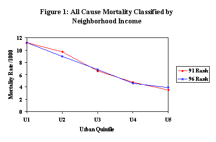
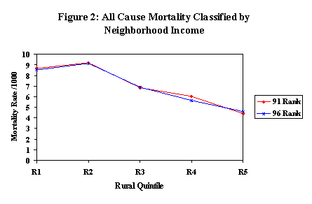
Mortality Rate by 1996 Census Ranking versus 1991 Census Ranking

To test whether the magnitude of association between income quintile and health measures has changed, we compared the mortality rate by 1996 census income quintile to the mortality rate by 1991 census income quintile. Figures 1 and 2 below, illustrate the relationship between all-cause mortality rate and income quintile. In each graph, there are two data series: one reports the mortality rate for each of five quintiles where both deaths and denominator populations are ranked using the 1991 census income quintile classification. The second series ranks the exact same death events and population counts according to the 1996 census. In both the urban and rural income quintile classification, there is no evidence of important differences in either point estimates or slope.

As a secondary point of some importance, figure 2 shows that the expected linear slope in mortality in relation to income is not present in the lowest rural income quintile. We found that this anomaly was due to age differences in the rural quintiles. After age-adjustment the expected slope is restored.

Mortality Rate Excluding PCH Residents

We also compared the relationship between all-cause mortality and income quintile excluding residents of a personal care home using the personal care home system files. As discussed previously, postal codes where 90% or more of the population is in a personal care home are excluded from the ranking procedure and defined as unrankable. However this exclusion does not remove all PCH residents from being ranked (see table below). Of the population resident in a personal care home in December 1994 (9,223) about 35% - 37% are excluded by the postal code exclusion (2,259 by 1991 census income quintile and 3,461 by 1996 census income quintile). A comparison of the mortality rate including PCH residents (except those excluded by the postal code exclusion) to the mortality rate explicitly excluding PCH indicates that the inclusion or exclusion of PCH residents may affect the income quintiles differentially. The inclusion of PCH residents inflates the mortality rate in income quintile R2 and U2 by 22-24% and inflates the mortality rate in income quintile R5 and U5 by 6-8%. Programmers and investigators should carefully consider the effect of the inclusion of PCH residents to their problem when using income quintiles.

Table 5: A Comparison of Mortality Rates Determined by Inclusion and Exclusion of PCH - 1991

Census Income Quintile	All-Cause Mort.	Mort. to PCH Residents	Total Pop	Pop in PCH	Rate Incl PCH	Rate Excl PCH	Ratio
Total	9,390	2,085	1,152,651	9,223	8.15	6.39
Out of Prov Muncode	113	0	0	0	.	.
Out of Prov Postal Code	13	2	409	1	31.78	26.96
Personal Care Home	764	731	3,528	3,259	216.55	122.68
Other Institution	271	159	2,913	913	93.03	56.00
Postal Code Missing Income	197	140	2,941	592	66.98	24.27
Muncode Missing Income	5	1	254	0	19.69	15.75
Postal Code not present on PCCF	28	2	7,725	10	3.62	3.37
Rural Q1	521	76	60,237	288	8.65	7.42	1.17
Rural Q2	547	109	59,455	407	9.20	7.42	1.24
Rural Q3	404	37	58,991	183	6.85	6.24	1.10
Rural Q4	381	47	63,067	187	6.04	5.31	1.14
Rural Q5	266	16	60,546	99	4.39	4.14	1.06
Urban Q1	1,838	235	164,393	947	11.18	9.81	1.14
Urban Q2	1,530	294	170,762	1,192	8.96	7.29	1.23
Urban Q3	1,105	114	166,327	549	6.64	5.98	1.11
Urban Q4	761	73	165,591	334	4.60	4.16	1.10
Urban Q5	646	49	165,512	262	3.90	3.61	1.08

Table 6: A Comparison of Mortality Rates Determined by Inclusion and Exclusion of PCH - 1996

Census Income Quintile	All-Cause Mort.	Mort. to PCH Residents	Total Pop	Pop in PCH	Rate Incl PCH	Rate Excl PCH	Ratio
Total	9,390	2,085	1,152,651	9,223	8.15	6.39
Out of Prov Muncode	113	0	0	0	.	.
Out of Prov Postal Code	13	2	409	1	31.78	26.96
Personal Care Home	823	786	3,838	3,461	214.43	98.14
Other Institution	271	159	2,913	913	93.03	56.00
Postal Code Missing Income	32	8	2,152	74	14.87	11.55
Muncode Missing Income	9	1	467	0	19.27	17.13
Postal Code not present on PCCF	0	0	32	0	0.00	0.00
Rural Q1	523	83	61,269	308	8.54	7.22	1.18
Rural Q2	566	107	61,814	429	9.16	7.48	1.22
Rural Q3	436	47	63,316	207	6.89	6.16	1.12
Rural Q4	330	28	58,666	133	5.63	5.16	1.09
Rural Q5	278	21	60,622	99	4.59	4.25	1.08
Urban Q1	1,874	273	167,570	1,060	11.18	9.62	1.16
Urban Q2	1,635	308	167,530	1,324	9.76	7.98	1.22
Urban Q3	1,104	129	167,498	563	6.59	5.84	1.13
Urban Q4	802	97	167,448	492	4.79	4.22	1.13
Urban Q5	581	36	167,107	159	3.48	3.26	1.07

Small Population Areas as a Possible Source of Variation

In a small number of geographic areas, the difference between the 1991 census average household income value and the 1996 census average household income value is quite large. To examine whether these differences are associated with small population areas, we looked at the correlation of population and percent change ((1996 Average Income - 1991 Average Income) / 1996 Average Income). The degree of correlation is very low (see table 7 below).

Table 7: Correlation of Population and Percent Change

Category	Number of Geographic Units	Correlation Coeff. between Percent Change and Population
All Postal Codes/Municipality Codes Present in 1991 and 1996	19,003	.013
Excluding Postal Codes/Municipality Codes with Imputation	18,282	.011

Secondly we divided all of the geographic units present in 1991 and 1996 into 20 groups (each with approximately 950 geographic units) with the lowest population geographic units in group 1 and the highest population geographic units in group 20. The mean and the standard error of the percent change is tabled below.

Table 8: Analysis of PCH Percent Change - 91 versus 96

Group	NObs	Mean	Std Error	Minimum	Maximum
1	950	0.0199009	0.0070385	-2.4185973	0.5763451
2	950	0.0261762	0.0059552	-1.8509420	0.6872895
3	950	0.0355564	0.0063220	-3.1080960	0.5763451
4	950	0.0354675	0.0059671	-1.5093409	0.5763451
5	950	0.0379873	0.0056920	-1.0885943	0.4583986
6	950	0.0434513	0.0055247	-1.0271157	0.6080207
7	950	0.0480757	0.0053374	-1.0885943	0.6080207
8	950	0.0422116	0.0057483	-1.1799900	0.4278862
9	950	0.0489787	0.0054501	-1.0885943	0.6080207
10	950	0.0490371	0.0048732	-1.1147996	0.5763451
11	950	0.0570640	0.0048269	-0.8201969	0.5527369
12	950	0.0494452	0.0050704	-1.1147996	0.5763451
13	950	0.0499932	0.0052908	-1.6776295	0.5435160
14	950	0.0457394	0.0051186	-1.1229384	0.6016932
15	950	0.0429267	0.0063064	-3.1080960	0.3970343
16	950	0.0468442	0.0045502	-0.9032973	0.5527369
18	950	0.0461901	0.0048495	-1.0926426	0.5375326
19	950	0.0383308	0.0055291	-0.9685047	0.5763451
20	950	0.0264660	0.0065912	-1.2976509	0.5435160

There is no real evidence of interdependence between the population size of the geographic unit and the percent difference between the 1991 average household income value and the 1996 average household income value in any of this analysis.

Final Words and Cautions

The 1996 census income quintile performs in a similar fashion as the 1991 census income quintile. The following are some important final notes about the income quintile ranking method.


• The income quintile uses a neighborhood measure of average household income to rank observations. Individual and household level measures of average household income are not generally available due to confidentiality concerns.
  
  
• First Nations people living in strictly urban areas (as defined by the 1996 PCCF) will be ranked by postal code. All others will be assigned an income quintile on the basis of their home reserve, regardless of whether they actually live on the reserve. This cannot be overcome since Treaty Status Indians always maintain their home reserve municipality code whether they live there or not. For this reason, income quintile rankings of treaty First Nations may not be very good.
  
  
• Portions of any event data set will not be ranked for various reasons as described in the income quintile ranking method above.
  
  
• The urban/rural definition used in this work is based upon a Statistics Canada definition of urban or rural (see Division of Data into Strictly Urban, Mixed Urban/Rural and Strictly Rural Postal Codes above). As a result populations living on the periphery of Winnipeg, for example, may be defined as rural by the census.
  
  
• Only personal care home residents living in postal codes where 90% or more of the population is in a personal care home are excluded from the income quintile ranking. Other personal care home residents present in an event file will be ranked (appropriately or inappropriately).
  
  
• While income is stratified by geography in urban areas pretty well, this may not be the case in rural areas. As a result, the relationship between health measures and income is often much stronger in urban areas than in rural areas.

References

- Mustard CA, Derksen S, Berthelot JM, Wolfson M, Roos LL. Age-specific education and income gradients in morbidity and mortality in a Canadian province. Soc Sci Med 1997;45(3):383-397. [Abstract] (View)
- Mustard CA, Frohlich N. Socioeconomic status and the health of the population. Med Care 1995;33(12 Suppl):DS43-DS54. [Abstract] (View)
- Roos NP, Mustard CA. Variation in health and health care use by socioeconomic status in Winnipeg, Canada: does the system work well? Yes and no. Milbank Q 1997;75(1):89-111. [Abstract] (View)
Request information in an accessible format
If you require access to our resources in a different format, please contact us:
- by phone at 204-789-3819
- by email at info@cpe.umanitoba.ca
We strive to provide accommodations upon request in a reasonable timeframe.
Contact us
Manitoba Centre for Health Policy
Rady Faculty of Health Sciences,
Room 408-727 McDermot Ave.
University of Manitoba
Winnipeg, MB R3E 3P5 Canada